This will be my attempt of trying to predict whether passengers on the titanic survived or died aboard the titanic. I will be using the famous titanic dataset available from Kaggle This analysis will be done in R.

To start off I will load the datasets in and have a look at the variables and try to make sense of them.

library(kntir)
train <- read.csv(train.csv)
test <- read.csv(test.csv)
str(train)

‘data.frame’: 891 obs. of 12 variables: $ PassengerId: int 1 2 3 4 5 6 7 8 9 10 … $ Survived : int 0 1 1 1 0 0 0 0 1 1 … $ Pclass : int 3 1 3 1 3 3 1 3 3 2 … $ Name : Factor w/ 891 levels “Abbing, Mr. Anthony”,..: 109 191 358 277 16 559 520 629 417 581 … $ Sex : Factor w/ 2 levels “female”,”male”: 2 1 1 1 2 2 2 2 1 1 … $ Age : num 22 38 26 35 35 NA 54 2 27 14 … $ SibSp : int 1 1 0 1 0 0 0 3 0 1 … $ Parch : int 0 0 0 0 0 0 0 1 2 0 … $ Ticket : Factor w/ 681 levels “110152”,”110413”,..: 524 597 670 50 473 276 86 396 345 133 … $ Fare : num 7.25 71.28 7.92 53.1 8.05 … $ Cabin : Factor w/ 148 levels “”,”A10”,”A14”,..: 1 83 1 57 1 1 131 1 1 1 … $ Embarked : Factor w/ 4 levels “”,”C”,”Q”,”S”: 4 2 4 4 4 3 4 4 4 2 …

The dataset is fairly small and contains only 12 variables. Our target variable here is Survived which takes the value 1 if the passenger survived and 0 if they did not. A priori, we can make some guesses about what variables might impact survival. It looks like factors such as sex, age and gender would likely affect chances of survival. After all, having seen the movie, women and children were the first to get on boats so surely that would make them more likely to survive. The variable Pclass indicates what class passengers were in. It seems reasonable to assume that passengers in 1st class had priorty to getting a lifeboat.

Alright, lets actually start looking at the data to see if it supports any of these theories. I am using the knitr library as it makes nice tables in the console for our summary stats.

library(knitr)
kable(summary(train[,1:5]))
kable(summary(train[,7:12]))

INSERT TABLE HERE

Looking at the summary stats, we can see that some of the variables are missing a lot of values. We will need to deal with this later if we want to have any decent kind of prediction. There are a few things we can do in this case such as dropping the NA observations (probably not a good idea), mean imputation (perhaps) or we can use a package called mice in R which basically imputes data using random forests. This latter approach is probably the approach I will take as it uses the other data to predict the missing values.

Next we start to look at some plots using the ggplot2 library. We might as well start by seeing how many people actually survived versus how many died. If an overwhelming amount died then we may have class imbalances and need to adjust our data by under or over sampling to make the number of people surviving and not surviving approximately equal.

library(ggplot2)
table(train$Survived)
barplot(table(train$Survived),names.arg = c('Perished', 'Survived'),
main = 'Died or Survived', col = 'blue')

ggplot(train, aes(x =  Sex, y = Age, fill = Sex)) + geom_boxplot()

ggplot(train, aes(as.factor(Pclass), fill=as.factor(Survived)))+ 
  geom_bar()

ggplot(train, aes(as.factor(Sex), fill=factor(Survived)))+geom_bar()


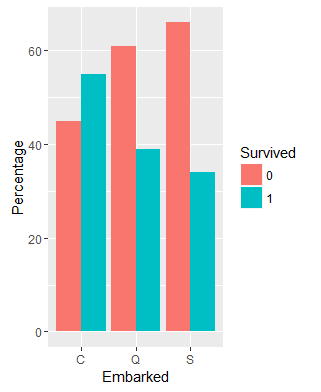
ggplot(train[train$Embarked != '',], aes(x = Embarked), fill=as.factor(Survived))+geom_bar()


ggplot(train, aes(as.factor(Pclass), fill=as.factor(Survived)))+geom_bar()

ggplot(train, aes(x = SibSp, fill = factor(Survived))) +
  geom_bar(stat='count', position='dodge') +
  scale_x_continuous(breaks=c(1:11)) +
  labs(x = 'Siblings')

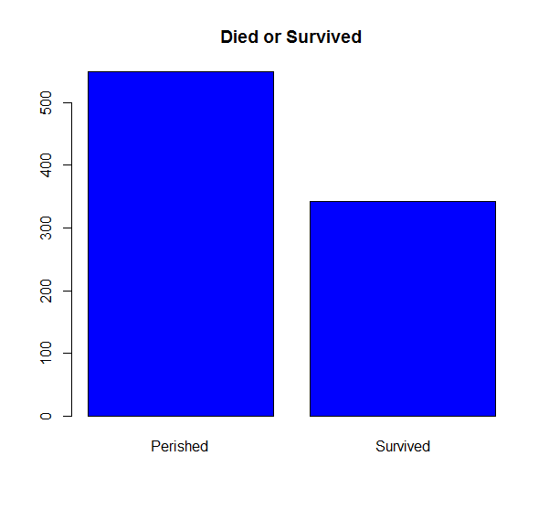
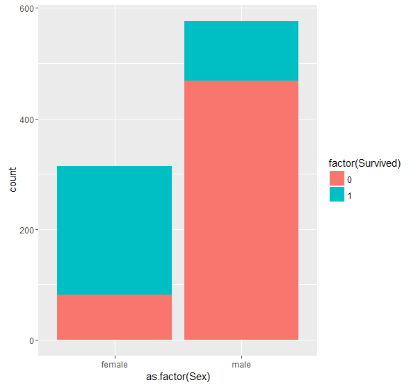
The graphs suggests that 549 people did not survive while 342 survived. This is approximately balanced and should not cause any major problems for prediction. Next we plot the number of males and females aboard while also looking at the proportions who survived. The plot tells us two things. First, there was approximately twice as many males on board than females and second, that males were actually much more likely to not survive than females. Presumably this is due to women and children having precedence for boarding life boats.

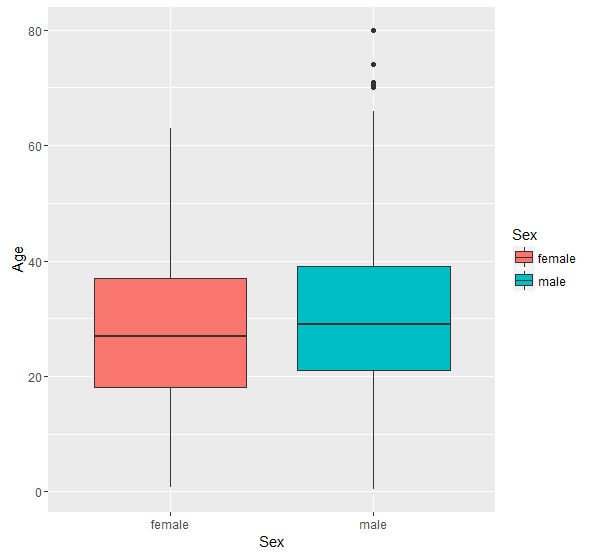
Next up I try looking at Sex by age via a boxplot and see if anything interesting pops out. First of all, It appears that the median age for men is higher than for women. It also looks like there were a number of older men on board in their 70’s. We might get improved results by getting rid of these outliers. We will replace these by the median Age for males later.

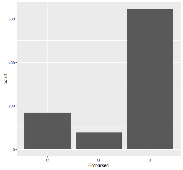
The Embarked variable tells us where the passenger got on. After a quick look up on the Internet I found out that the three categories C,Q and S stand for Cherbourg, Queenstown, Southamption respectively. From the graph, it looks like the majority of passengers got on at Southampton. We can see that for both S and Q the number of passengers who did not survive exceeds the number of passengers who did survive. This was not the case in C however, where the proportion of people that survived was larger than the proportion who did not. Im not quite sure why this is the case.

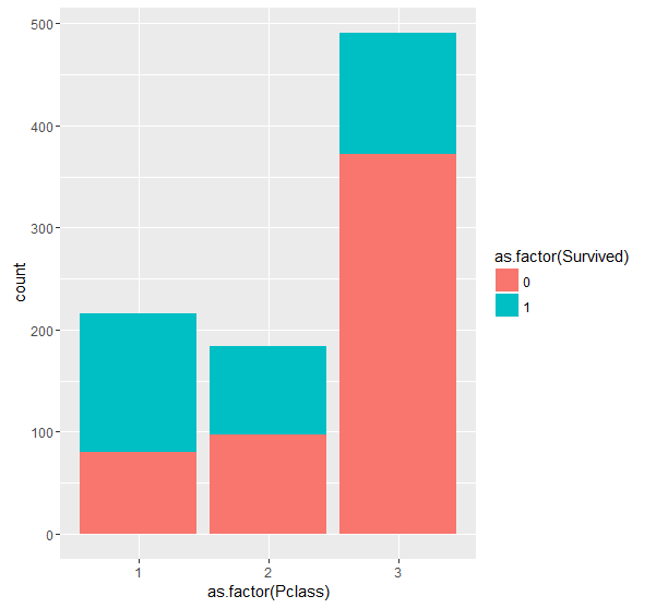
The last plot we will have a look at before we begin cleaning and organizing the data is that of passenger class. In the description of the data on Kaggle, this variable is listed as a proxy for social class with Pclass = 1 meaning upper class. One would think that being in a higher class means you are more likely to survive as you might get priority in the lifeboats? Let’s see if this is the case.

From the graph, it appears that being in Pclass one makes you marginally more likely to survive than to not survive. Likewise, being in the lowest class (Pclass 3) made someone significantly more likely to perish. As well as being more likely to get priority on a lifeboat, this could have also been due to location on the ship since I believe that lower class passengers were given rooms further below deck which likely impacted their ability to escape in time.

Ok, I think that’s enough for our EDA. We can now start messing around with the data a little bit and do some feature engineering. Before, we get into that however, I am going to join the training and test set together so that any changes we make in terms of features or filling in missing values will be made to both. We can split them up again before training our model on them. We must create a Survived column in the test set to make the dataframes the same size before we append the rows of both datasets. This is simple enough to do in R.

Survived = train$Survived
test$Survived = NA
train_new = rbind(train, test)

toFactor <- function(data) {
   columns <- intersect(names(data), c("Survived", "Sex", "Embarked";, "Pclass", "Ticket"))
  data[, columns] <- lapply(data[, columns] , factor)
  return(data)
}

train_new <- toFactor(train_new)

We also make a simple function that transforms all our categorical variables to factors. The first thing we need to think about is the missing values in the dataset. To give us a nice visual representation we can use a nice package in R called Amelia.

library(Amelia)
missmap(train, main="Titanic Training Data - Missings Map", col=c("yellow", "darkgrey"), legend=FALSE)

summary(train$Age) 

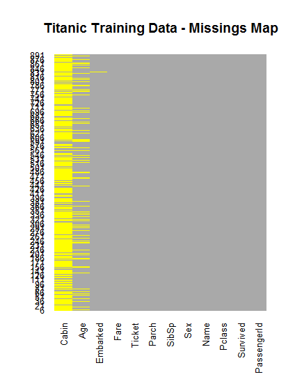
We are missing a number of observations for Age and especially cabin. As I mentioned before there are a number of ways to deal with missing data. The Age variable could perhaps be imputed using some of the other variables. For example, we could use a persons title in their name to infer their age or least to infer the likely range of their age. Perhaps the best way to proceed though, is to use a machine learning algorithm to predict the values. The MICE package in R implements this quite easily using a random forest to predict a persons age using the other available information. We will use this to predict the empty values in Age and Embarked. After reading through the Kaggle forums, I found a very interesting approach of how to fill in the missing values of Cabin which I will probably try at a later date.

Since Embarked only has two missing values we will fix this first. One thing we could do is just fill in S for both of these since it is the most common point of departure and there is a relatively high chance that these passengers left from here. Let’s use the MICE package, however, since it will use more information and hopefully come up with a better prediction. We are going to use the following variables in our random forest:

Age, Sex, Fare, PClass, SibSp, Parch, Embarked, Title. Below is the code to estimate this.

library(mice)
set.seed(111)
indv = c("Sex" "Fare", "Pclass", "SibSp", "Parch", "Embarked", "Title")
result <- mice(train_new[, names(train_new) %in% indv], method = 'rf')

out = complete(model)
out[missingEm,]
train_new$Embarked =  out$Embarked

Pclass	Sex	SibSp	Parch	Fare	Embarked
1	female	0	0	80	S
1	female	0	0	80	S

As it happens, our fancy algorithm predicts the exact same as our mode imputation.Another way I could do this would be to look at the median fare of passenger classes from each of the different cities. It looks like the median fare in C tend to be around the $80 mark and so makes it more likely that these passengers embarked from there. We could go with either method but for the moment I will just go with the results from the random forest.

embark_fare <- full %&gt;%
filter(PassengerID != 62 & PassengerID != 83

ggplot(embark_fare, aes(x = Embarked, y =Fare, fill = factor(Pclass))) +
geom_boxplot() + 
geom_hline(aes(yintercept = 80),
color = 'red' , linetype = 'dashed', lwd = 2) +
scale_y_continous(labels=dollar_format()) +
theme_few()

Now we will start on the feature engineering section of our analysis. I will come back to the Age variable and fill in the missing values when I have made some changes to the dataset. Looking at the name variable, we probably only need the title rather than the whole name. We will need to do some text manipulation here to extract only the title from the string. The R library stringr will be very helpful here. We will use the str_split function from this package which makes it very easy to extract what we need. It appears that the data in the Name column is in the following form

1. Braund, Mr. Owen Harris
2. Cumings, Mrs. John Bradley (Florence Briggs Thayer)
3. Heikkinen, Miss. Laina
4. Futrelle, Mrs. Jacques Heath (Lily May Peel)
5. Allen, Mr. William Henry
6. Moran, Mr. James

If this is the case for all rows then we can split the sentence into two by splitting on the comma (,). This will be stored in a list and we want the second part of the list. Once we have that we need to split again, this time on the full stop. We then extract the first item from this second list and this will be ‘Mr’ in the case of the first example above.

This can be wrapped in an sapply to apply it to every row in the data. Now here is the code to perform this. Btw we store this in a new variable in the train_new dataset called Title. After we check for the unique titles which may help us fill in some of the missing ages.

train_new$Title <- sapply(train_new$Name, function(x) str_split(x, ', ')[[1]][2])
train_new$Title <- sapply(train_new$Title, function(x) str_split(x, '. ')[[1]][1])

unique(train_new$Title)

We can load a library called Hmisc and use the bystats function to give us a nice table which provides an overview of the missing values of Age by title.

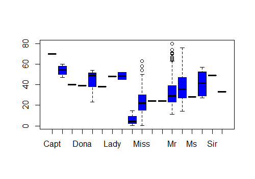
It looks like we are missing a lot of values from Mr and Mrs and Miss. We are also missing values from Master. After a quick look on Wikipedia we see that the definition of Master is a male under the age of 12. This is going to be helpful for filling in our missing age for Master. I perform a boxplot to give me an idea of the distribution of ages for all Titles. It looks like there are a few passengers with the title Master over 12. Let’s look at the max value for Master.

library(Hmisc)
bystats(train_new$Age, train_new$Title,
fun = function(x) c(Mean = mean(x), Median = median(x)))

temp = train_new[train_new$Title =='Master',]
max(na.omit(temp$Age))

This gives us a max age of 14.5 for Master. Now I am going to move on and try and reduce the number of categories contained in the title variable making use of the Age and Sex variables. We are going to create the following groups. Mr for men above 14.5 years old. Master for boys below and equal to 14.5 years. Miss for girls below and equal to 14.5 years. Ms for women above 14.5 years, maybe unmarried. Mrs for married women above 14.5 years I am also going to give any unique or uncommon male names the “Mr” title so we have a more concise set of title categories. I do a similar exercise for the female names such as “Lady” and “The Countess”. The code below implements these changes.

train_new[(train_new$Title == "Mr" &amp; train_new$Age <= 14.5 &amp; !is.na(train_new$Age)),]$Title = "Master"

train_new[train_new$Title == "Capt"|
train_new$Title == "Col"|
train_new$Title == "Don"|
train_new$Title == "Major"|
train_new$Title == "Rev"|      
train_new$Title == "Jonkheer"|
train_new$Title == "Sir",]$Title = "Mr"

train_new[train_new$Title == "Dona"|
train_new$Title == "Mlle"|
train_new$Title == "Mme",]$Title = "Ms"


train_new[train_new$Title == "Lady"| train_new$Title == "the Countess",]$Title = "Mrs"

# Categorise doctors as per their sex
train_new[train_new$Title == "Dr" &amp; train_new$Sex == "female",]$Title = "Ms"
train_new[train_new$Title == 'Dr' &amp; train_new$Sex == 'male',]$Title = 'Mr'

I then define these new title categories as factors and provide a quick summary table. The result of this data cleaning gives us a much more concise categorical variable that contains the name information but will be easier for our model to make sense of when training.

Master Miss Mr Mrs Ms 66 260 777 199 7

Ok we can leave this variable alone for now and move on. Next we are going to have a look at the SibSp and Parch variables. We can use these variables to make a new family variable, where it’s value will be equal to the number of Siblings (SibSP) plus the number of Parents (Parch) + one (individual). We can then go further and separate into small versus large families as maybe larger families were less likely to survive. Let’s plot this and see what we find.

ggplot(train, aes(x = SibSp, fill = factor(Survived))) +
  geom_bar(stat='count', position='dodge') +
  scale_x_continuous(breaks=c(1:11)) +
  labs(x = 'Siblings')

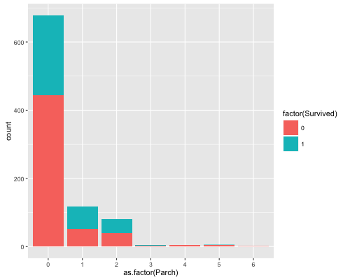
ggplot(train, aes(x = as.factor(Parch), fill = factor(Survived))) + geom_bar()

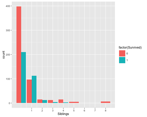
We can see from the Siblings graph, passengers with more siblings such as 5-8 had a 100 per cent non-survival rate. This might be useful, especially if we categories into big and small families. Ok this will be slightly arbitrary but I am going to define a family as small if it has 3 or less people.

As well as this, I am going to create a variable called mother which will be a “Mrs” who has a family size of greater than one. This is basically being driven by the whole women and children first concept. If this indeed did happen on the titanic then its stands to reason that a women with a child will be more likely to survive all else equal.

train_new$FamilySize <- ifelse(train_new$SibSp + train_new$Parch + 1 <= 3,1,0)

train_new$Mother <- ifelse(train_new$Title == 'Mrs' &amp; train_new$Parch &gt; 0,1,0)

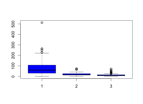
Next up, we are going to try and do something with the Fare variable. Assuming people who paid large fares were relatively wealthy and were probably of a higher societal class, they may have been more likely to survive. Having a look at the fare class it looks like there are 13 observations that seemed to pay nothing for their ticket. Now I am not really sure why this is the case but perhaps they won a place on the maiden voyage?

Plotting Fare by Pclass reveals that indeed passengers in 1st class paid higher median fares. Likewise passengers in 3rd class paid much less and in fact were more likely to not survive. Since the 0 values seem to be evenly spread through the Pclasses I will just impute the median value. I do the same for the one NA value as well.

boxplot(train_new$Fare ~ train_new$Pclass, col = 'blue')

train_new[which(train_new$Fare == 0), ]$Pclass
train_new$Fare[which(train_new$Fare == 0)] = median(train_new$Fare, na.rm = TRUE)
train_new$Fare[which(is.na(train_new$Fare))] = median(train_new$Fare, na.rm = TRUE)

I am going to do is split the Age variable into smaller categories instead of having it as a continuous variable. This may help prediction later on. Before I do that, however, I will perform a random forest to impute the missing values of Age.

age.df <- mice(train_new[, !names(train_new) %in% 
c("Survived","Name","PassengerId","Ticket","AgeClass","Cabin","SibSp", "Parch")],
m=8,maxit=8,meth='pmm',seed=123)

ggplot(train_new,aes(x=Age)) + 
  geom_density(data=data.frame(train_new$PassengerId, complete(age.df,6)), alpha = 0.2, fill ="blue")+
  geom_density(data=train_new, alpha = 0.2, fill ="Red")+
  labs(title="Age Distribution")+
  labs(x="Age")

train_new_imp <- data.frame(train_new$PassengerId, complete(age.df,6))
train_new$Age = train_new_imp$Age

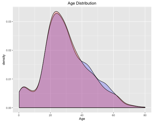
Plotting the Age distribution reveals that our imputations keeps approximately the same distribution which is good. Finally, I split ages up into 4 categories which will hopefully cause our model to perform better.

train_new$AgeClass <- ifelse(train_new$Age < 10,1, 
ifelse(train_new$Age &gt; 10 &amp; 
train_new$Age <= 20, 2, 
ifelse(train_new$Age &gt; 20 &amp; 
train_new$Age < 35,3,4)))
train_new$AgeClass <- as.factor(train_new$AgeClass)

That’s it for part 1 of this little project. I may come back and do a little more with the data. I found some really helpful posts and ideas on Kaggle that I may try out with regards making use of the cabin variable. In part 2 I will focus on training a few different models on the data and testing how accurate they are. Look forward to that. Any comments or suggestions are welcome.