This is the second part of the Titanic Kaggle Competition. In this part I will train a few different models on our new dataset and see what kind of results we get. The first thing I need to do is split my data back up into training and test sets. Having a quick look at the data, the test set begins in row 892 where the Survived row is equal to NA and so we split the dataset here. I also take a random 90 10 split on the training set so I can test how well my models are doing before I submit them to kaggle.

train  = train_new[1:891,]
test = train_new[892:1309,]

train$gp <- runif(dim(train)[1])
testSet <- subset(train, train$gp  <= 0.1)
trainingSet <- subset(train, train$gp &gt; 0.1)

Ok, now I am going to run my first model. For classification problems I usually like to start out with a simple logistic regression model and use that as a benchmark. This is simple enough to implement in R using the glm function with the family = binomial argument. Our dependent variable is of course Survived and our independent variables will be the following: Sex, AgeClass, Pclass, FamilySize, Fare, Mother, Embarked and Title

reg1 <- glm(Survived ~ Sex + AgeClass + Pclass +
FamilySize + Title + Fare + Mother + Embarked, family = binomial(link = 'logit') ,
data = trainingSet)
summary(reg1)

It seems like the most significant variables from this logistic regression are Pclass, AgeClass = 4,Family Size and the title Mr. This is a good start and it shows us that at least some of our variables have some predictive ability for survival. Next I test how accurate this model is on the 10 per cent holdout test set. The code is below.

We get an accuracy of 0.7692 on our test set. Not the most phenomenal score in the world but it’s a start and it beats some of the benchmark scores on kaggle. This will be a useful benchmark to try and beat.

fitted.results <- predict(reg1, newdata = testSet, type = 'response')
fitted.results <- ifelse(fitted.results &gt; 0.5,1,0)

misClasificError <- mean(fitted.results != testSet$Survived)
print(paste('Accuracy',1-misClasificError))

We could next try a logistic regression with an L2 penalty also known as a Ridge regression. Below is an equation implementing an L2 penalty term. It works be penalising the squared norm of the coefficients w. If overfitting is occurring then this will help to minimise it.

$ l(w) = ln \prod P(y^j | x^j,w) - \lambda \lVert \mathbf{w} \rVert_2^2 $

I am going to digress a bit here to discuss overfitting which is a very common problem when training models and is a very important concept to understand and recognise. To see why this L2 penalty term works consider the following. Imagine we had a model that linearly separated our data. In other words it perfectly identified all positive outcomes (all survivors) correctly and all negative outcomes (all non survivors) correctly. Although ostensibly this looks like it is a very good model, in reality it probably isn’t. The reason being is that our model has more than likely overfit the training data. This kind of overfitting in logistic regression tends to happen when we include higher order terms in our regression, Age squared or Age cubed for example. It causes our decision boundary to become more complicated. See for example the graphs below which I kindly borrowed from coursera Andrew Ng’s Machine learning course on Coursera, a great course for anyone interested btw. The graphs show the decision boundary under different order polynomial terms.

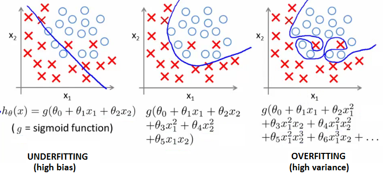
We can see that as we add higher order terms to our independent variables our decision boundary starts to become more complicated. In the case of a squared term, the predictor actually looks pretty good. In the case of the graph on the far right, however, our classifier has perfectly identified all of our positive and negative examples. The main danger with this is that our model will likely generalize poorly to new data and end up making poor predictions.

So how can we identify overfitting?

Having near perfect accuracy on our training set is a sure fire sign of overfitting. Another one of the tell tale signs of overfitting in logistic regression is large coefficients. Consider a 2 dimensional example where we have a linear decision boundary that perfectly separates the positive and negative examples. Our equation would be as follows:

$ \hat{w}_1 #positive - \hat{w}_2 #negative = 0 $

In this case the equation of our decision boundary line would equal 0 as above. Now imagine we multiple each side by some constant, say 10. Well our coefficients have gotten 10 times bigger but this decision boundary also separates the data perfectly since it is also equal to 0. This is true for any value of the coefficients. The reason the coefficients become large is a symptom of maximum likelihood. To understand why, we need to recall that the goal of maximum likelihood is to find the coefficients which maximise the probability of correctly identifying the target variable.

For example, if we substitute a coefficient value of 0.5 into our sigmoid function we get an estimated probability of 0.62 (See below). In other words our model thinks there is a 62 per cent chance our prediction is correct. if however, we scale up our coefficients by 10 like before, we get an estimated probability of .99. We are now 99 per cent confident that we have a positive outcome. In fact as the model becomes more and more complex the parameter values go to infinity.

$\frac{1}{1+e^-0.5} = 0.62$

$\frac{1}{1+e^-5.0} = 0.99$

Our L2 term means that we are now trying to minimise a cost function which contains the magnitude of the coefficients. Now we can see why our L2 term essentially penalises large coefficients by making our overall cost function larger.

Btw since we are not using any higher order polynomial terms here we are not overfitting with this particular logistic regression, however, this is very easy to do with decision trees and random forests and so will be more applicable for the other models we will be using. For illustration purposes though I find that overfitting is easier to understand in the context of logistic regression.

Below I show the code to run our L2 regularised logistic regression. I am using the glmnet library in R to do this. One of the things we need to decide is the value we will give to our regularization parameter lambda. We have to strike a balance between a value that is not too big which will shrink our parameters too much and cause the error to increase and a value that is not too small where very little regularization is occurring. A simple way to chose is to perform cross validation using the cv.glmnet function. We pass a series of lambda values (generated with our grid variable) to this function and it runs a series of logistic models models using each parameter as its L2 penalty value. We then choose the lambda value which minimizes the Residual Sum of Squares.

library(glmnet) 
x.m = data.matrix(trainingSet[,c(3,5,6,10,12,13,14,15,16)])
y.m = trainingSet$Survived

grid=10^seq(10,-2,length=100)
cvfit.m.ridge = cv.glmnet(x.m, y.m,
family ="binomial", 
alpha = 0,lambda = grid,
type.measure ="class")

coef(cvfit.m.ridge, s ="lambda.min")


pred2 = predict(cvfit.m.ridge, 
s = 'lambda.min', 
newx=data.matrix(testSet[,c(3,5,6,10,12,13,14,15,16)]), 
type="class")

misClasificError_ridge <- mean(pred2 != testSet$Survived)
print(paste('Accuracy',1-misClasificError_ridge))

Once we have extracted our minmimum value of lambda we can run our L2 regularised logistic regression model on our training set and see how well it does at prediction. It turns out that this model actually performs worse than our first model which probably just highlights the fact that our model was not overfit.

The next algorithm that I will try is a random forest. These algorithms tend to perform fairly well for these kinds of problems and so I expect to get an improvement over the logistic model.

Here is the code:

library(randomForest)
set.seed(111)

rf1 <- randomForest(as.factor(Survived) ~ Pclass +
Sex + Fare + Embarked +
Title + FamilySize +
Mother + AgeClass
,data = trainingSet,
importance = TRUE,
ntree = 2000)

importance <- importance(rf1)
VarImportance <- data.frame(Variables = row.names(importance),
Importance = round(importance[, 'MeanDecreaseGini'],2))

rankImportance <- VarImportance %>% 
mutate(Rank = paste0('#', dense_rank(desc(Importance))))

ggplot(rankImportance, aes(x = reorder(Variables, Importance),
y = Importance, fill = Importance)) +
geom_bar(stat = 'identity') + geom_text(aes(x = Variables, y = 0.5, label = Rank),
 hjust = 0, vjust = 0.55, size = 4, color = 'red') +
labs(x = 'Variables') +
coord_flip()         

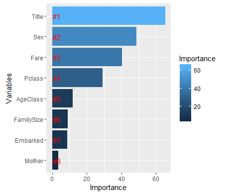
In the code above I load in the randomForest library and train my model on the same set of variables as the other models. I tried a few different values for the number of trees and they don’t really seem to make much of a difference so I settle on ntrees = 2000. I also use the importance function as this allows me to see the relative importance of each of the variables in the model.

From the graph below it looks as though the most important variable is the title variable. This highlights the gains to be made from feature engineering. Other important variables include Sex, Fare and Pclass which we highlighted during the EDA phase of the analysis.

When we submit this model on Kaggle our score does indeed improve. Our score on the public leaderboard with this model is 0.799904. I definitely think this score can be improved. The next step would be to go back to the feature engineering phase and use some of the data we didn’t take advantage of before. We never used the Cabin variable since there were so many missing values. Looking at the kaggle forums, there are some clever approaches people have used to use create a new Deck variable with the cabin data.

After seeing a layout of the titanic it looks as though the letter in front at the start of the cabin variable corresponds to the deck. Now you would think that decks closer to either the main deck of the ship or lifeboats would make it more likely for passengers to survive. So this approach could yield pretty good results. Another interesting idea is to create a feature based on whether or not your family survived and you could work this out by looking at passengers surnames. I suspect that adding these kind of features would improve my score and I will likely revisit this analysis in the future and try to move up the leaderboard. For the moment, though, that it is. Thanks for reading and feel free to leave any questions or comments.