Today I am going to implement a Bayesian linear regression in R from scratch. This post is based on a very informative manual from the Bank of England on Applied Bayesian Econometrics. I have translated the original matlab code into R for this post since its open source and more readily available. Hopefully, by the end of this post, it will be clear how to undertake a Bayesian approach to regression and also understand the benefits of doing so.

Ok lets get started. Ordinarily, If someone wanted to estimate a linear regression of the matrix form:

$Y_t = B X_t + \epsilon_t$

$\epsilon_t \sim N(0,\sigma^2)$

They would start by collecting the appropriate data on each variable and form the likelihood function below. They would then try to find the $ B $ and $ \sigma^2 $ that maximises this function.

$ F Y_t B,\sigma^2 = (2\pi \sigma^2)^{-T/2} \exp(- \frac{(Y_t-B X_t)^T (Y_t-B X_t)}{2 \sigma^2}) $

In this case the optimal coefficients can be found by taking the derivative of the log of this function and finding the values of $\hat{B}$ where the derivative equals zero. If we actually did the math, we would find the solution to be the OLS estimates below. I will not go into the derivation here but here is a really nice video going through deriving the OLS estimates in detail.

$\hat{B} = (X_t’ X_t)^{-1}(X_t’ Y_t)$

and we would find our variance equal to

$\sigma^2 = \dfrac{\epsilon’ \epsilon}{T}$

where T is the number of rows in our dataset. The main difference between the classical Frequentist approach and the Bayesian approach is that the parameters of the model are solely based on the information contained in the data whereas the Bayesian approach allows us to incorporate other information through the use of a prior. We are able to incorporate this prior belief by using Bayes rule. Remeber the forumla for Bayes rule is

$ p(A|B) = \frac{P(B|A) \times P(A)}{P(B)} $

We can apply this formula to describe the posterior distribution of our parameters (what we want to find) in the following way.

$ H(B,\sigma^2 Y_t) \propto F(Y_t B, \sigma^2) \times P(B,\sigma^2) $

This equation states that the posterior distribution of our parameters conditional on our data is proportional to our likelihood function (which we assume is normal) multiplied by the prior distribution of our coefficients. There is usually a term $F(Y)$ in the denominator on the right hand side (equivalent to the P(B) in Bayes rule) but since this is only a normalising constant to ensure our distribution integrates to 1. Notice also that it doesn’t depend on our parameters so we can omit it for the moment.

In order to calculate the posterior distribution, we need to isolate the part of this posterior distribution related to each coefficient. This involves calculating marginal distributions, which for many models in practice is extremely difficult to calculate analytically. This is where a numerical method known as Gibbs sampling comes in handy. The Gibbs sampler let’s us use draws from the conditional distribution to approximate the joint marginal distribution. Here is a quick overview of how it works:

Imagine we have a joint distribution of N variables: $ f(x_1, x_2, \dots ,x_N) $ and we want to find the marginal distribution of each variable. If the form of these variables are unknown, however, it may be very difficult to calculate the necessary integrations analytically. In cases such as these, we take the following steps to implement the Gibbs algorithm. First, we need to initialise starting values for our variables, $ x_1^0 \dots x_N^0 $

Next we sample our first variable conditional on the current values of the other N-1 variables. i.e. $f(x_1^1 | x_2^0, \dots , x_N^0) $. We then sample our second variable conditional on all the others $f(x_2^1 |x_1^1, x_3^0, \dots , x_N^0)$ , repeating this until we have sampled each variable. This ends one iteration of the Gibbs sampling algorithm. As we repeat these steps a large number of times the samples from the conditional distributions converge to the joint marginal distributions. Once we have M runs of the Gibbs sampler, the mean of our retained draws can be thought of as an approximation of the mean of the marginal distribution.

Now that we have the theory out of the way, let’s see how it works in practice. Below I will show the code for implementing a linear regression using the Gibbs sampler. In particular, I will estimate an AR(2) model on US Gross Domestic Product (GDP). I will then use this model to forecast GDP growth and make use of our Bayesian approach to construct confidence bands around our forecasts using quantiles from the posterior density i.e. quantiles from the retained draws from our algorithm.

Our model will have the following form:

$Y_t = \alpha + B_1Y_{t-1} + B_2Y_{t-2} + \epsilon_t$

We can also write this in matrix form by defining the following matrices. $B = [\alpha_1,B_1,B_2]’$ which is just a vector of coefficients, and our matrix of data $X_t = [1,Y_{t-1}, Y_{t-2}]’$. This gives us the form in equation 1 up above. The goal here is to approximate the posterior distribution of our coefficients $\alpha,B_1,B_2$ and $\sigma^2 $. As discussed above, we can do this by calculating the conditional distributions within a Gibbs sampling framework. Ok so let’s start coding this up in R.

The first thing we need to do is load in the data. For simplicity I am going to use the quantmod package in R to download GDP data from the Federal Reserve of St.Louis (FRED) website. I also transform it into growth rates.

library(quantmod)
getSymbols("GDPC96", src = "FRED")
data = <- na.omit(UNRATE)
p = 2

data <- 100*(diff(log(data))
data <- data[-1,] # lose one obs after differencing

We get rid of any ‘NA’ data using the na.omit function and we define 2 lags of our variable (p=2). Next we define a function to create our X matrix which contains our lagged GDP rate and a constant term. This is a nice function to have as if you are doing any sort of matrix algebra you will need to organise your matrices into a form similar to this.

BregData <- function(data,p,constant){

  nrow <- as.numeric(dim(data)[1])
  nvar <- as.numeric(dim(data)[2])
  
  Y1 <- as.matrix(data, ncol = nvar)
  X <- embed(Y1, p+1)

  X <- X[,(nvar+1):ncol(X)]
  if(constant == TRUE){
     X <-cbind(rep(1,(nrow-p)),X)
    }
  Y = matrix(Y1[(p+1):nrow(Y1),])
  nvar2 = ncol(X)

 return = list(Y=Y,X=X,nvar2=nvar2,nrow=nrow) 
}

Our function takes in three parameters. The data, the number of lags and whether we want a constant or not. We could also augment this function to include a trend term as well. I won’t though for this particular analysis. The function returns our new matrices and their new dimensions.

Our next bit of code implements our function and extracts the matrices and number of rows from our results list. We are also going to set up our priors for the Bayesian analysis.

results = list()
results <- BregData(data,p,TRUE)

X <- results$X
Y <- results$Y
nrow <- results$nrow

B0 <- c(0,0,0)
B0 <- as.matrix(B0, nrow = 1, ncol = nvar)
sigma0 <- diag(1,nvar)

T0 = 1       # prior degrees of freedom
theta0 = 0.1     # prior scale

B = B0
sigma2 = 1
reps = 10000

What we have done here is essentially set a normal prior for our Beta coefficients which have mean = 0 and variance = 1. For our mean we have priors:

$\begin{pmatrix} \alpha_0
B^0_1
B^0_2
\end{pmatrix} = \begin{pmatrix} 0
0
0 \end{pmatrix}$

And for our variance we have priors:

$\begin{pmatrix} \Sigma_a & 0 & 0
0 & \Sigma_{B1} & 0
0 & 0 & \Sigma_{B2}
\end{pmatrix} = \begin{pmatrix} 1 & 0 & 0
0 & 1 & 0
0 & 0 & 1
\end{pmatrix}$

For sigma, we have set an inverse gamma prior. $p(\sigma^2)\sim \Gamma^{-1} (\dfrac{T_0}{2}, \dfrac{\theta_0}{2})$. For this example, we have arbitrarily chosen T0 = 1 and theta0 = 0.1. These are often, however, set to small values in practice (Gelman 2006). We could do robustness tests by changing our initial priors and seeing if it changes the posterior much. If we try and picture changing our theta0 value, a higher value would essentially give us a wider plot with our coefficient being more likely to take on larger values in absolute terms, similar to having a large prior variance on our Beta.

Now we initialise some matrices to store our results. We create a matrix called out which will store all of our draws. It will need to have rows equal to the number of draws of our sampler, which in this case is equal to 10,000. We also need to create a matrix that will store the results of our forecasts. Since we are calculating our forecasts by iterating an equation of the form:

$Y_t = \alpha + B_1Y_{t-1} + B_2Y_{t-2} + \epsilon_t$

We will need our last two observable periods to calculate the forecast. This means our second matrix out1 will have no. of forecast periods + number of lags, 14 in this case. We will also define our main function that calculates the Gibbs sampling algorithm in the next code snippet.

out = matrix(0, nrow = reps, ncol = nvar + 1)
colnames(out) <- c('constant', 'beta1','beta2', 'sigma')
out1 <- matrix(0, nrow = reps, ncol = 14)

gibbs_sampler <- function(X,Y,B0,sigma0,sigma2,T0,D0,reps,out,out1){
  
k = ncol(X)
T1 = nrow(X)

#Main Loop
for(i in 1:reps){
  M = solve(solve(sigma0) + as.numeric(1/sigma2) 
  * t(X) %*% X) %*% (solve(sigma0) %*%
  B0 + as.numeric(1/sigma2) * t(X) %*% Y)
  
  V = solve(solve(sigma0) + as.numeric(1/sigma2) *
    t(X) %*% X)
  
  chck = -1
  while(chck < 0){   # check for stability
    
    B <- M + t(rnorm(3) %*% chol(V))
    b = matrix(c(B[2], 1, B[3], 0), nrow = k-1, ncol = k-1)
    ee <- max(sapply(eigen(b)$values,abs))
    if( ee<=1){
      chck=1
    }
  }
  # compute residuals
  resids <- Y- X%*%B
  T2 = T0 + T1
  theta1 = theta0 + t(resids) %*% resids
  
  #draw from Inverse Gamma
  z0 = rnorm(T1,1)
  z0z0 = t(z0) %*% z0
  sigma2 = theta1/z0z0
  
  # keeps samples after burn period
  out[i,] <- t(matrix(c(t(B),sigma2)))
  
  # compute 12 month forecasts
  yhat = rep(0,14)
  end = as.numeric(length(Y))
  yhat[1:2] = Y[(end-1):end,]
  cfactor = sqrt(sigma2)
  for(m in 3:14){
    yhat[m] = c(1,yhat[m-1],yhat[m-2]) %*% B + 
    rnorm(1) * cfactor
  }
  out1[i,] <- yhat
}
  return = list(out,out1)
}


results1 <- gibbs_sampler(X,Y,B0,sigma0,sigma2,T0,D0,reps,out,out1)

coef <- results1[[1]][9001:10000,]
forecasts <- results1[[2]][9001:10000,]

OK so this is a big complicated looking piece of code but I will go through it step by step and hopefully it will be clearer afterward. First of all, we need the following arguments for our function. Our initial variable, in this case, GDP Growth(Y). Our X matrix, which is just Y lagged 2 periods with a column of ones appended. Next we need all of our priors that we defined earlier, the number of times to iterate our algorithm (reps) and finally, our 2 output matrices. The main loop is what we need to pay the most attention to here. This is where all the main computations take place. Line 12 to 15 calculates M and V. These are the posterior mean and variance of $ B $ conditional on $ \sigma^2 $. I won’t derive these here, but if you are interested they are available in Time Series Analysis Hamilton (1994). To be explicit, the mean of our posterior parameter Beta is defined as:

$ M = (\Sigma_0^{-1}+ \dfrac{1}{\sigma^2}X_t’X_t)^{-1}(\Sigma_0^{-1}B_0 + \dfrac{1}{\sigma^2}X_t’Y_t) $

and the variance of our posterior is defined as:

$ V = (\Sigma_0^{-1}+ \dfrac{1}{\sigma^2}X_t’X_t)^{-1} $

If we play around a bit with the second term in M, we can substitute our maximum likelihood estimator for $ Y_t $. Doing so gives us

$ M = (\Sigma_0^{-1}+ \dfrac{1}{\sigma^2}X_t’X_t)^{-1}(\Sigma_0^{-1}B_0 + \dfrac{1}{\sigma^2}X_t’X_tB_{ols}) $

Essentially this equation says that M is just a weighted average of our prior mean and our maximum likelihood estimator for Beta. If for example, we assigned a small prior variance, we are imposing the restriction that our posterior will be close to the prior and the distribution will be quite tight.

After calculating the 3x1 vector of Coefficients $B$ by generating 3 random variables from the normal distribution, We then transform them using our mean M and variance V at each iteration. The next bit of code also has a check to make sure the coefficient matrix is stable i.e. our variable is stationary which ensures our model is dynamically stable. By recasting our AR(2) as an AR(1), we can check if the absolute values of the eigenvalues are less than 1. If they are, then we can be sure our model is dynamically stable. This eigenvalue method can be used for any sized AR or VAR model.

Now that we have our draw of $B$, we draw sigma from the Inverse Gamma distribution conditional on $B$. To sample a random variable from the inverse Gamma distribution with degrees of freedom $\dfrac{T}{2}$ and scale $\dfrac{\theta}{2}$ we can sample T variables z0 from a standard normal distribution and then make the following adjustment $ z = \dfrac{\theta}{z0’z0}$. z is now a draw from the correct Inverse Gamma distribution.

The next line (38) stores our draws of the coefficients into our out matrix. We then use these draws to create our forecasts below this. The code essentially creates a matrix yhat, to store our forecasts for 12 periods into the future. Remember, we need a matrix of size 14 because we are using an AR(2) which requires using the last 2 observable data points. Our equation for a 1 step ahead forecast can be written as

$ \hat{Y}{t+1} = \alpha + B_1 \hat{Y}{t} + B_2 \hat{Y}_{t-1} + \sigma v^* $

In general, we will need a matrix of size n+p where n is the number of periods we wish to forecast. The forecast is just an AR(2) model with with a random shock each period that is based on our draws of sigma. That is it for the algorithm. All we need to do is run the function and look at the results. The code below extracts the coefficients that we need which correspond to the columns of the coef matrix. Each row gives us the value of our parameter for each draw of the gibbs algorithm. Calculating the mean of each of these variables gives us an approximation of the empirical distribution of each coefficient. if we wanted to we could use these distribution for hypothesis testing.

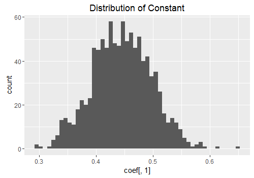
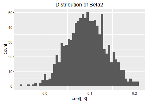
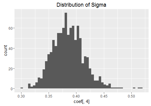
Below I have plotted the posterior distribution of the coefficients. Notwithstanding a few outliers, they resemble a normal distribution. If we did enough draws of the algorithm, these figures would start to look more and more like the familiar bell shape of the normal distribution.

const <- coef[,1]
beta1 <- coef[,2]
beta2 <- coef[,3]
sigma <- coef[,4]

const_mean <- mean(const)
beta1_mean <- mean(beta1)
beta2_mean <- mean(beta2)
sigma_mean <- mean(sigma)

coef_means <- c(const_mean,beta1_mean,beta2_mean,sigma_mean)

forecasts_mean <- as.matrix(colMeans(forecasts))

library(ggplot2)
qplot(coef[,1], geom = "histogram", bins = 50, main = 'Distribution of Constant')
qplot(coef[,2], geom = "histogram", bins = 50,main = 'Distribution of Beta1')
qplot(coef[,3], geom = "histogram", bins = 50,main = 'Distribution of Beta2')
qplot(coef[,4], geom = "histogram", bins = 50,main = 'Distribution of Sigma')

Since we are doing a Bayesian analysis, I decided to create a forecast with confidence bands around it. I found a very helpful BOEblog online which creates fancharts for forecasts very similar to the Bank of Englands Inflation reports. I make use of the fanplot library here and I adapted the code for my particular data which results in the plot below. It took a bit of playing around with some of the options to get a graph that looked reasonably nice so you may have to mess around with some of the values to get the aesthetic look you are after.

library(fanplot)
forecasts_mean <- as.matrix(colMeans(forecasts))
forecast_sd <- as.matrix(apply(forecasts,2,sd))
tt <- seq(2017, 2019.75, by = .25)
y0 <- 2017
params <- cbind(tt, forecasts_mean[-c(1,2)], forecast_sd[-c(1,2)])

p <- seq(0.05, 0.95, 0.05)
p <- c(0.01, p, 0.99)

k = nrow(params)
gdp <- matrix(NA, nrow = length(p), ncol = k)

for (i in 1:k) 
  gdp[, i] <- qsplitnorm(p, mode = params[i,2], 
  sd = params[i,3])


plot(GDP, type = "l", col = "tomato", lwd = 2, 
xlim = c(y0 - 5, y0 + 3), ylim = c(-1, 2), 
xaxt = "n", yaxt = "n", ylab="")

## background
rect(y0 - 0.5, -2 - 1, y0 + 3, 3 + 1, 
border = "gray90", col = "gray90")


fan(data = gdp, data.type = "values", probs = p, 
start = y0-0.25, frequency = 4, 
anchor = GDP[time(GDP) == y0 - 0.50], 
fan.col = colorRampPalette(c("tomato", "gray90")),  
ln = NULL, rlab = NULL)


## BOE aesthetics
axis(2, at = -1:2, las = 2, tcl = 0.5, labels = FALSE)
axis(4, at = -1:2, las = 2, tcl = 0.5)
axis(1, at = 2012:2019, tcl = 0.5)
axis(1, at = seq(2012, 2019, 0.25), labels = FALSE, tcl = 0.2)
abline(h = 0)  #boe cpi target
abline(v = y0 + 1.75, lty = 2)  #2 year line

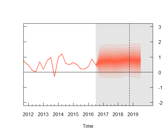
The confidence bands are pretty large as you can see and so, not surprisingly using an AR(2) model may not be the best choice. I am sure better models could be created by incorporating more variables into a Vector Auto Regression framework but I think this is fine for the purposes of an introduction to Bayesian estimation.